


What will a camera measure when the imaging conditions change?
To answer this, we usually rely on suppliers’ specifications and optical design software to choose an instrument, before validating it on our own samples in controlled, fixed setups. Such standard characterization gives essential measurements, but each one describes a single set of conditions. Change the lighting, the sample or the viewing geometry, and new effects appear, from sample metamerism [1] and instrument chromatic aberrations [2] to changes in measured color caused by the combined effects of illumination, optics and sensor response [3]. Testing every combination on a physical bench quickly becomes impractical.
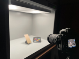
Figure1 : a characteristic validation setup
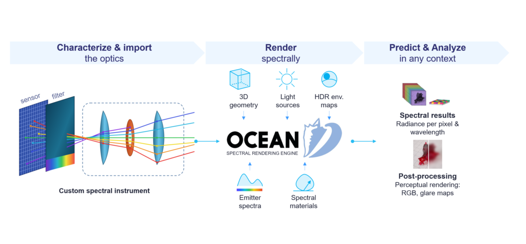
Our approach is to make the optical system part of the spectral rendering pipeline (Fig. 2). You characterize your optics of interest once and upload that characterization into Ocean™, which then lets you explore as many configurations as you need, without going back to the bench.
Importantly, Ocean™ does not import your optics: you do not provide the lens design to the renderer. Instead, our software creates a model of the system’s behavior, built from the measurements you provide. This is what makes the approach work for instruments whose internal design is unknown, confidential, or too complex to reproduce.
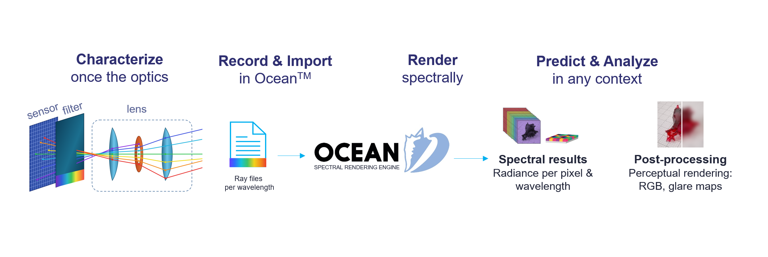
Figure 2 : Overview of our custom instrument integration in Ocean™
To make this possible, we extend a physically based camera model [4] with wavelength-dependent optical behavior. The model captures both the geometric and the chromatic response of the optical system, fits different users’ workflows, and stays numerically efficient. This article presents the main steps and gives a rough description of each. The full details are in our proceedings [5].
Building a virtual spectral camera in Ocean™
1) Characterizing the optical system
Choose your optics. The first step is to select the optics of your camera and characterize its behavior. You can choose among different types of lens (Fig. 3):
- a lens you designed yourself, in software such as Code V, RayJack One or Optiland
- a black-box lens imported in Zemax, which reproduces the manufacturer’s specifications while its internal design stays hidden from the user
- an analytical model, such as an ideal thin lens [7].
Any optics that is rotation-invariant can be chosen.
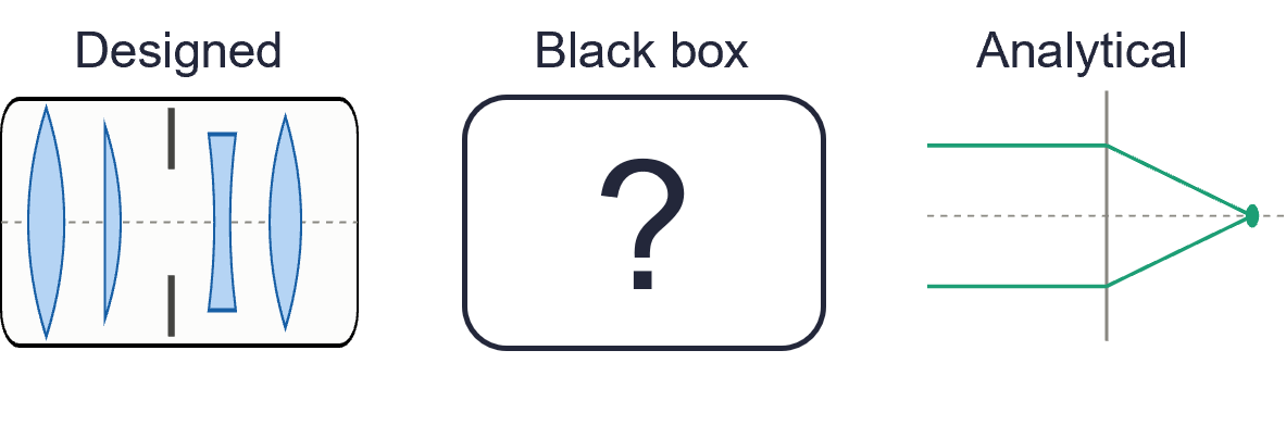
Figure 3 : Different optics that can be considered for simulation in OceanTM.
2) Generating ray files trough optical ray tracing
Trace rays through the system. Next, in your chosen third-party software, trace rays as they travel through the optics[1] (Fig. 4, left). The exit pupil must be fully sampled to ensure an accurate implementation in Ocean™. To fit your workflow, two sampling strategies are possible (Fig. 4, right):
- Beam sampling: rays are emitted from the input plane (the sensor side of the optics). For each position Pᵢ, several directions Dᵢ are generated. The rays that pass through the system are collected on the output surface.
- Ray sampling: a single direction is used for each ray position. Rays can be emitted and collected in either direction, from sensor to scene side or the other way around[2].
[1] Taking advantage of the rotation invariance of the optics, only one direction needs to be explored. Thus, rays origin can be defined in terms of input plane’s off-axis distance along one axis.

[2] Ray sampling allows users to generate rays in the scene-to-sensor direction, before rotating and reversing rays directions to obtain rays from input to output surfaces.
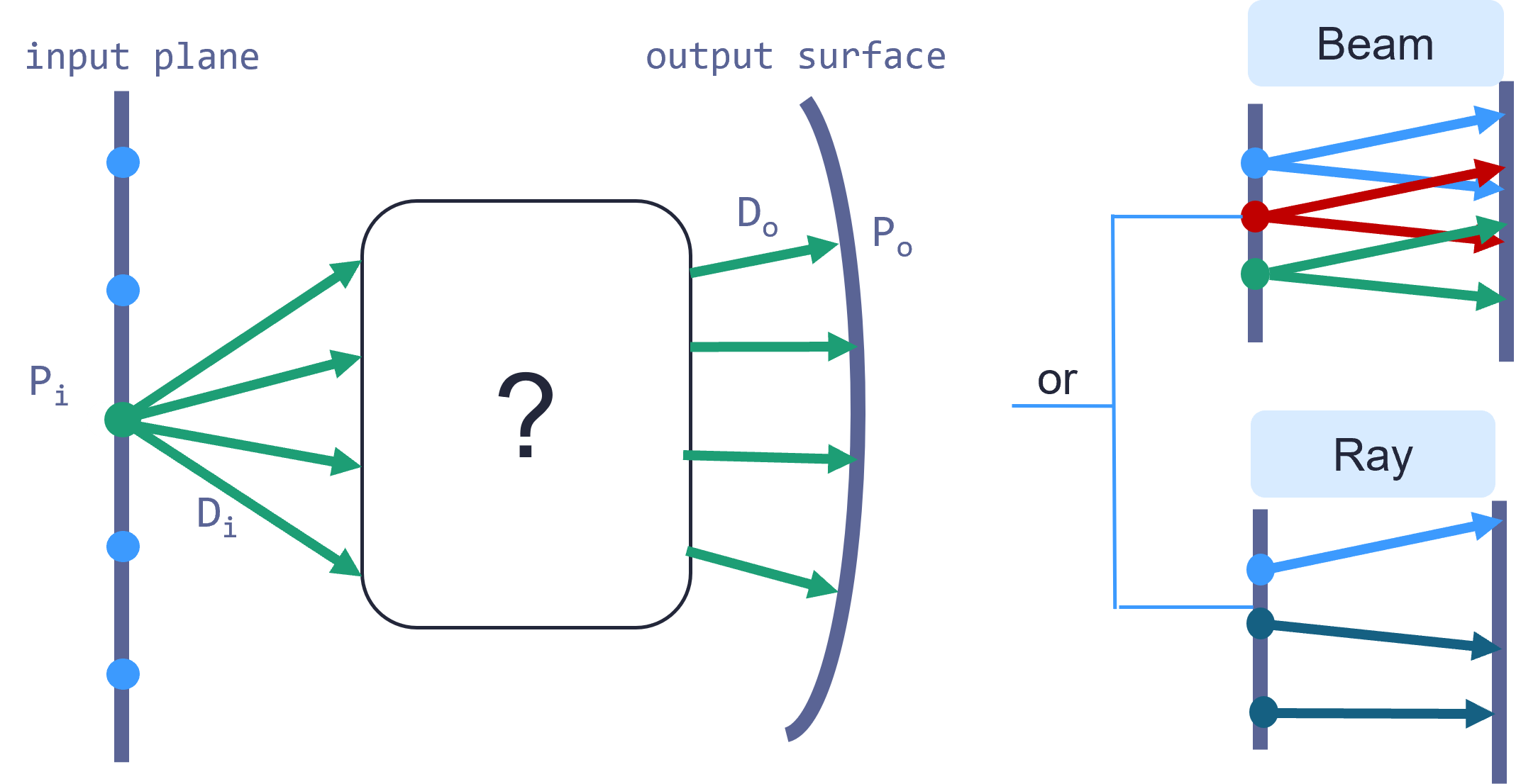
Figure 4: Tracing rays from input plane to output surface to create ray files. Two approaches, beam or ray sampling, can be used.
Record the ray files. Finally, the passing rays are saved in ray files (Fig. 5, example files available [7,8]), one per wavelength explored. Each file contains a header describing the characterization, followed by the list of ray positions and directions on the input plane and on the output surface.
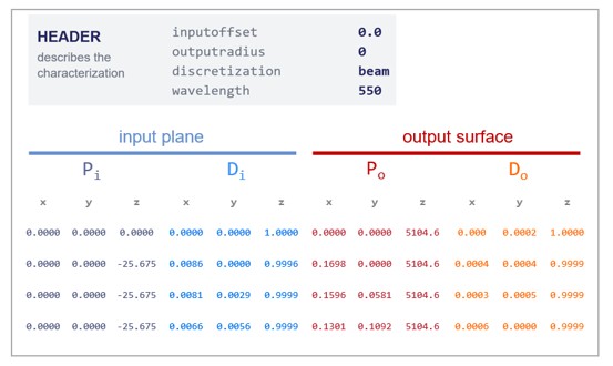
Figure 5: Ray file structure. (Example files can be downloaded on Zenodo [9])
3) Importing Ray Files into Ocean™
Ray Files. In the spirit of the BSDF converter that loads your measurement and create the corresponding material, Ocean™ now features a CAM importer that loads your ray files and creates the associated instrument. From the data provided, Ocean™:
- fits Ray Transfer Functions (RTFs) [4], which describe via a multi-variate polynomial how rays would be redirected if they were traced through the optics (Figure. 6, left);
- derives Vignetting Functions from the collected passing rays, which describe mathematically[1] the set of rays that physically make it through the system (Figure 6, right).
Together, they keep rendering numerically efficient and restricting path tracing to the rays that should physically be considered.
a. Global and Local Ray Transfer Functions
Global or local RTFs. At import, you choose how the RTFs are generated:
- Global: a single set of functions applies to all rays.
- Local: the input plane is partitioned into spatial regions, each with its own RTF. During rendering, each RTF is applied to the rays that originate in that region.
The two strategies trade accuracy against computational cost, both when generating the RTFs and during rendering. Our paper [5] discusses this trade-off in detail [2].
[1] For each beam off-axis position, or subset of rays position, rays successfully transmitted through the optical system are projected onto a pass-plane located at some distance from the input plane. The boundary of the resulting ray distribution is approximated by an ellipse [12] whose parameters depend on the off-axis distance considered.

[2]  Global RTF formulation is robust to irregular datasets but may require significant computational time to generate for large polynomial degree and large ray files. In contrast, although more sensitive to dataset sparsity, the local strategy reduces the generation time and can achieve comparable accuracy using lower-degree polynomials.
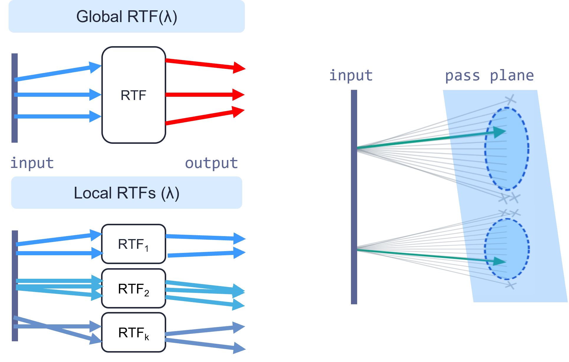
Figure 6: Importing ray files, two types of ray transfer functions can be generated (left) and vignetting functions are determined (right).
b. Optional illumination correction
Illumination curve (optional). You can add an illumination curve [4,10] to correct for subtle effects that the vignetting functions do not capture. The curve describes the relative irradiance fall-off as a function of the distance from the sensor center (the off-axis distance), with the optics in focus. It can be generated with the same software used to characterize the optics. This illumination correction[1] can also be added in a post-processing step.
c. Modeling angle- and wavelength-dependent sensor filters
Sensor filter (optional). A spectral filter file can be uploaded to model a physical filter placed between the sensor and the lens. This filter modulates the intensity of rays reaching the sensor as a function of their incident angle and wavelength, via a transmission function T(λ,θs) (Fig. 7). The file contains a listing of the intensity factor T (between 0 and 1) for a set of wavelengths λ and sensor incidence angles θ. In Ocean™, this is called an Angle Variable Spectrum, avspectrum , its construction is detailed in the documentation [13].
[1] Vignetting functions implemented only describe the mecanical blockage of rays. However, sensor illumination fall-off also results from more subtle effects [14]. Moreover, the elliptical approximation breaks down for complex optics [4]. Importing an illumination curves permits correcting as a post-processing step.
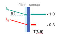
Figure 7: Sensor filter modulates rays’ intensity on the sensor via a transmission function T that depends on their incident angle θ and wavelength λ.
Configuring and Rendering with the Virtual Camera
Once your instrument is generated[1], you can tune the usual camera parameters: sensor dimensions, resolution, position, exposure time, spectral range and sensor type (RGB, XYZ, etc.). Then proceed as for any other Ocean™ scene: import the scene geometry, define the optical properties of the materials and the emitters, and render. The result is a physically based simulation of what your camera would measure, including the geometric and chromatic behavior of its optics. Note that since the lens system is not imported and only its characterization is used, effects that depend on the internal optical layout, such as intra-lens reflections and ghosting, are currently reproduced with the generated instrument.
[1] The RTFs and vignetting functions are assigned to your instrument when it is created. You can generate other ones and assign them to the same instrument, which replaces the previous ones.
Application 1: Testing windshield geometries for ADAS cameras, without the bench
An ADAS camera never looks at the world directly: it looks through a windshield. Its rake angle, curvature and thickness all change what the camera captures, adding distortion and chromatic effects to the image the perception algorithms must work with [14]. Comparing windshield designs on a physical bench means manufacturing each candidate and realigning the setup every time, which is slow and expensive. With the CAM Importer, this exploration moves into simulation.
a. Reproducing the physical camera setup
Step 1: Reproduce the bench. We replicated the experimental setup in Ocean™: the ADAS camera facing a checkerboard target (Fig. 8, left). The physical camera was characterized once with the workflow above. Ray files were generated by beam sampling the black-box description of the optics in Zemax, then a global RTF and vignetting functions were fitted and assigned to a custom instrument in Ocean™. Camera position and sensor settings were set to match the physical bench.
b. Validating the virtual camera against experimental measurements
Step 2: Validate the instrument. We rendered the checkerboard as seen by the virtual camera (Fig. 8, right) and compared it with the image acquired on the bench. We performed a quantitative comparison, based on Modulation Transfer Functions, that validates the accuracy of the virtual instrument. The full methodology and results are available in our paper [5].
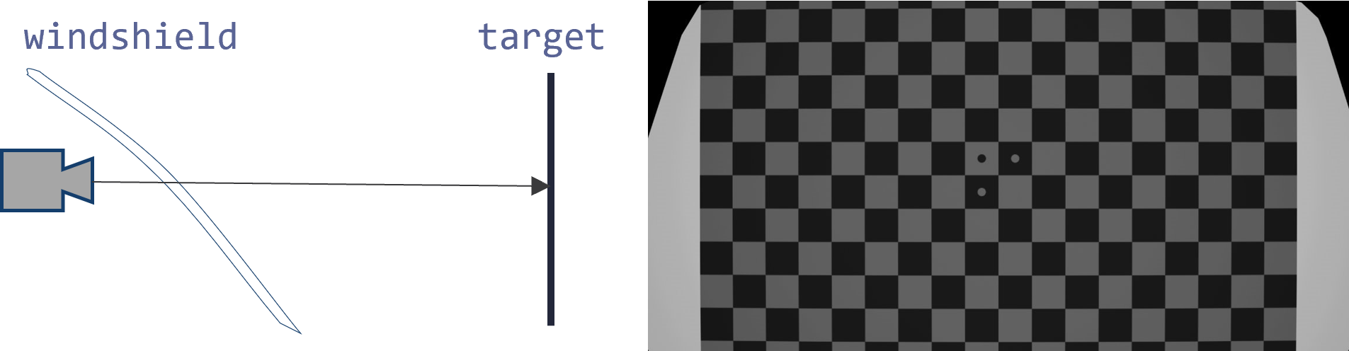
Figure 8: Left, experimental bench replicated in Ocean™. Right, simulated images of the checkerboard target.
c. Exploring windshield geometry in simulation
Step 3: Explore. With the instrument validated, the windshield can be added to the scene and its geometry (rake angle, curvature, thickness) varied freely, with no new characterization of the optics and no new prototype. Each configuration is simply a new render with the same custom instrument.
Application 2: Distinguishing metameric materials through optical design
Two surfaces can look exactly the same color to our eyes or to a camera, even though they reflect light very differently. This effect is called metamerism [1], and such pairs of materials are called metamers. Metamers are usually unmasked by changing the viewing conditions: lighting the pair with a different illuminant or placing spectral filters in front of the camera. Using our virtual spectral camera, we explore an alternative: telling metamers apart through the instrument itself, either with the chromatic aberration of its optics or with a purpose-designed sensor filter.
a. Building the virtual spectral camera
Step 1: Build the instrument. We created a virtual camera in Ocean™ from the same workflow as above, here with a simple optical design: an ideal thin lens that can be modelled analytically [7]. It is then given two variants (Fig. 9): a chromatic shift, where the lens focuses each wavelength at a slightly different distance (a Gaussian defocus centered on 650 nm, with a 30 nm width), and a sensor filter, where each pixel records a wavelength band depending on the angle at which light arrives (35 angular bins, ~9 nm spectral bands).
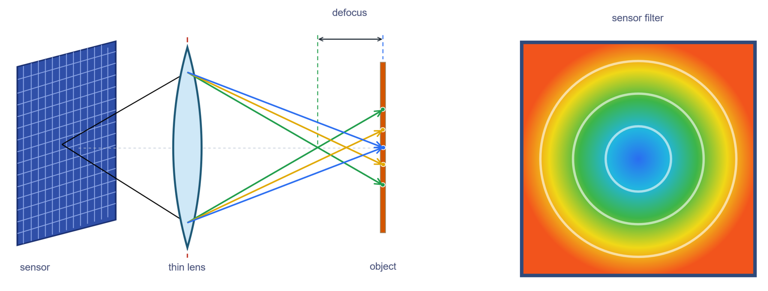
Figure 9: Left, Chromatic defocus introduced to the original ideal thin lens; Right, map of the wavelengths transmitted for different rays‘ incident angle on sensor
b. Establishing the baseline with metameric materials
Step 2: Set the baseline. We rendered a chip in a box lit by a D65 source placed on the top side of the box (Fig. 10, left). For the first simulation, we assign the sample with spectrum 1 from Fig. 9 and then spectrum 2 (Fig. 10, right). Through the ideal lens, the camera cannot tell the two materials apart: they appear identical (Figure 11, left).
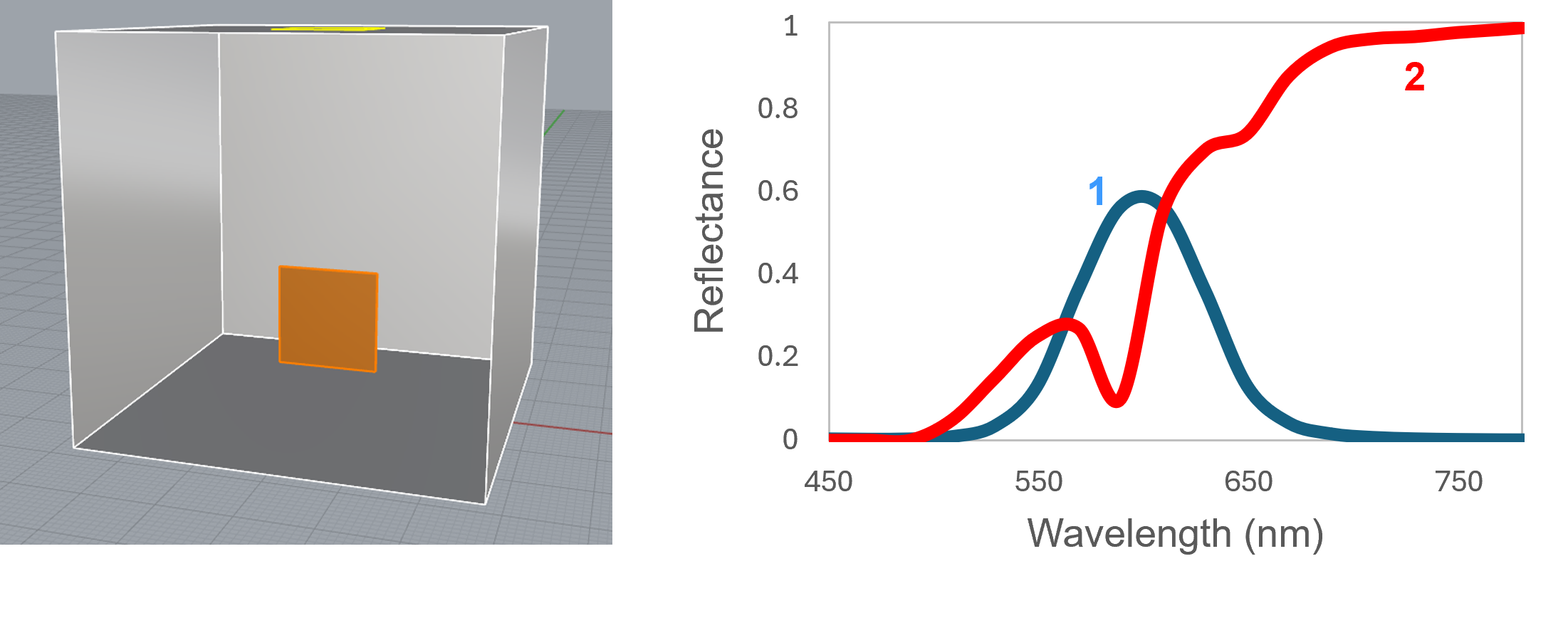
Figure 10: Left, 3D geometry of the scene considered; Right, spectra of the materials rendered.
c. Exploring chromatic aberration and sensor filters
Step 3: Explore. With the instrument defined, we only swap the optics by assigning a new RTF to the custom instrument, with no change to the scene. With the chromatic shift, each patch blurs differently around its edges because the lens defocuses the wavelengths where their spectra differ, and a color difference (ΔE CIE2000) appears between them (Fig. 11, middle). With the angle-dependent sensor filter, the two patches separate even more clearly (Fig. 11, right).
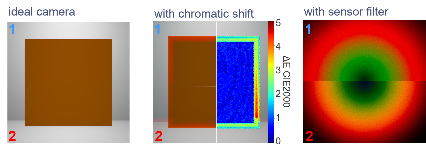
Figure 11: Rendered metamers with the ideal camera (left), camera with chromatic shift (middle), ideal camera with a sensor filter added (right).
Conclusion: From virtual camera validation to optical design exploration
Ocean™ can support both the validation of optical systems and the investigation of how optical behavior affects what a measurement system captures.
This work presented the CAM importer, explaining its operating principle and how it integrates custom instrument into Ocean™. By allowing users to import their own characterization data and use it to render the behavior of an optical system, the importer provides a flexible framework that can accommodate different instruments and user workflows. Rather than imposing a single characterization or simulation process, it enables users to leverage the data available to them and adapt the tool to their specific needs.
The first application demonstrates the validation of the CAM importer and custom instrument rendering. It provides a concrete example of how a digital twin can reduce the time and cost associated with experimental bench testing, while enabling flexible exploration of instrument configurations.
The second application explores a complementary opportunity: exploiting chromatic aberration as a potential source of spectral information rather than treating it solely as an optical defect to be corrected. Since different wavelengths can produce distinct spatial image patterns, the optical system itself may help discriminate between metamers that appear identical under conventional color measurements. This also opens new possibilities for optical design: by deliberately shaping a lens’s spectral response, could we improve material discrimination? The virtual spectral camera provides a means to investigate this question, compare alternative configurations, and assess their trade-offs before committing to a physical design.
Together, these applications illustrate how digital twins of optical systems can serve not only as tools for validating instrument models, but also as a means of exploring new measurement strategies and guiding optical design.
Flexible workflow: one characterization, infinite exploration:
1) Characterize the optical system
2) Generate ray files for the wavelengths of interest
3) Import the files into Ocean™
4) Fit ray transfer functions and derive vignetting functions
5) Configure the virtual camera and render the scene
6) Fine tune and validate the virtual camera reliably
Bibliographie
[1] Arash Akbarinia and Karl R. Gegenfurtner, “Color metamerism and the structure of illuminant space,” J. Opt. Soc. Am. A 35, B231-B238 (2018)
[2] W. J. Smith, Modern Optical Engineering: The Design of Optical Systems, 4th ed., McGraw-Hill, New York, 2008
[3] J. E. Farrell, F. Xiao, P. B. Catrysse, and B. A. Wandell, A simulation tool for evaluating digital camera image quality, Proc. SPIE Image Quality and System Performance, 5294, pg. 119–128 (2003)
[4] T. Goossens, Z. Lyu, J. Ko, G. C. Wan, J. Farrell, and B. Wandell, Ray-transfer functions for camera simulation of 3D scenes with hid den lens design, Opt. Express, 30(13), pg. 24031–24047 (2022).
[5] our CIC proceedings : Physically Accurate Spectral Camera Simulation and
Wavelength-Dependent Sensitivity Modelling
[6] Synopsys Inc., CODE V Optical Design Software, https://www.synopsys.com/optical-solutions/codev.html .
[7] R. Hartley and A. Zisserman, Multiple View Geometry in Computer Vision, 2nd ed., Cambridge University Press, Cambridge, 2003.
[8] Camera Importer: Ocean documentation
[9] Berthier, E., Tetaud, A., & Besse, G. (2026). Physically Accurate Spectral Camera Simulation and Wavelength-Dependent Sensitivity Modeling [Dataset]. In Physically Accurate Spectral Camera Simulation and Wavelength-Dependent Sensitivity Modelling. Zenodo. Color & Imaging Conference (CIC34), Barcelona, Spain. https://doi.org/10.5281/zenodo.22141550
[10] W. B. King, The approximation of vignetted pupil shape by an ellipse, Appl. Opt., 7(1), pg. 197–201 (1968).
[11] https://docs.eclat-digital.com/ocean2025-docs/nodes/filter/illuminance.html
[12] https://en.wikipedia.org/wiki/Vignetting
[13] https://docs.eclat-digital.com/ocean2025-docs/nodes/avspectrum.html
[14] BLASINSKI, HENRYK, FARRELL, JOYCE, LIAN, TRISHA, et al. “Optimizing image acquisition systems for autonomous driving”. Electronic Imaging 30 (2018), 1–7 1.

Q&A
What is a virtual spectral camera?
A virtual spectral camera is a computational model of an imaging system that reproduces its optical behavior using spectral rendering. In Ocean™, the model can account for wavelength-dependent optical effects using Ray Transfer Functions and vignetting functions derived from characterized optical behavior.
Can you simulate a camera without access to its internal lens design?
Yes. The CAM Importer in Ocean™ uses ray files generated from measured or simulated optical behavior, rather than requiring the internal lens design itself. This approach makes it possible to model optical systems whose designs are proprietary, unavailable or too complex to reproduce directly, provided suitable characterization data are available.
How is a virtual camera validated against a physical camera?
A virtual camera can be validated by reproducing an experimental setup in simulation and comparing the rendered images with measurements acquired using the physical instrument. In the ADAS camera application presented here, the experimental setup is replicated in Ocean™, and image quality is compared using Modulation Transfer Functions (MTFs).
How can spectral camera simulation help distinguish metameric materials?
Metameric materials can appear identical under a given illumination and measurement configuration despite having different spectral reflectance properties. By simulating wavelength-dependent optical behavior or an angle-dependent sensor filter, Ocean™ makes it possible to investigate whether these differences produce distinguishable image responses.
What data are required to create a virtual camera in Ocean™?
The workflow described in this article uses ray files generated by tracing rays through the optical system for the wavelengths of interest. These files contain ray positions and directions used by the CAM Importer to fit Ray Transfer Functions and derive vignetting functions. Optional illumination correction and sensor-filter data can also be included.


Responses